Uda Equation of Dirac Field @ Quantum History Theory @ Problems @ Forum @ www.GrammaticalPhysics.ac

since 2006
Help　Sitemap

< Forum >

< Problems >

< Quantum History Theory >

< Uda Equation of Dirac Field >

At first, I note down the every component of the matrices to be used.
　

σ₁σ₂ = -σ₂σ₁ = iσ₃, σ₂σ₃ = -σ₃σ₂ = iσ₁, σ₃σ₁ = -σ₁σ₃ = iσ₂,
σ₁σ₁ = σ₂σ₂ = σ₃σ₃ = σ₀.
　

[γ^μ, γ^ν]₊ = γ^μγ^ν + γ^νγ^μ = 2g^μν,
g⁰⁰ = 1, g¹¹ = g²² = g³³ = -1, μ≠ν ⇒ g^μν = 0.
When I was studying the Dirac equation, I did not think of noting down these details fully as necessary because I thought of such things as obvious.
So, now, a few decades after that, it has taken much effort for me to extract the above information.

The Hamiltonian H of the Dirac Field is as follows.
H = ∫d³x ψ†(x)γ⁰(-iγ^k∂_k + m)ψ(x)
Here (γ⁰γ^k)† = γ^k†γ⁰† = (-γ^k)(γ⁰) = -γ^kγ⁰ = γ⁰γ^k that is to say hermitian.
The quantization condition is as follows.
[ψ_α(x), ψ_β†(y)]₊ = δ_αβδ³(x - y),
[ψ_α(x), ψ_β(y)]₊ = 0.
The Schrodinger equation is as follows.
ih(d/dt)|Ψ_S(t)> = H|Ψ_S(t)>.

As a preparation, let's consider a quantum mechanics of two real degrees x, y of freedom.
H = c(x - iy)(x + iy),
[x + iy, x - iy]₊ ≡ (x + iy)(x - iy) + (x - iy)(x + iy) = 1,
[x + iy, x + iy]₊ ≡ (x + iy)(x + iy) + (x + iy)(x + iy) = 0.
ih(d/dt)|Ψ_S(t)> = H|Ψ_S(t)>
where c is real.

(x + iy)(x - iy) + (x - iy)(x + iy) = 2x² + 2y²
∴ x² + y² = 1/2

(x + iy)(x + iy) = x² - y² + i(xy + yx)
∴ [x, y]₊ = i(x² - y²) = i(2x² - 1/2) = i(1/2 - 2y²)

a ≡ x + iy, [a, a†]₊ = 1, [a, a]₊ = 0.

[a†a, a]_- = a†aa - aa†a = -aa†a = -(1 - a†a)a = -a,
[a†a, a†]_- = a†aa† - a†a†a = a†aa† = (1 - aa†)a† = a†.

a†a|n> = n|n>, <n|n> = 1.

a†aa|n> = 0 = 0a|n>　∵ aa = 0
(a|n>, a|n>) = <n|a†a|n> = n<n|n> = n
∴ a|n> = (√n)|0>

a†aa†|n> = (a†a†a + [a†a, a†]_-)|n> = [a†a, a†]_-|n> = a†|n> = 1a†|n>,
(a†|n>, a†|n>) = <n|aa†|n> = <n|(1 - a†a)|n> = (1 - n)<n|n> = 1 - n
∴ a†|n> = [√(1 - n)]|1>

n²<n|n> = (a†a|n>, a†a|n>) = <n|a†aa†a|n> = <n|a†(1 - a†a)a|n> = <n|a†a|n> = n<n|n>
∴ n² = n
∴ n(n - 1) = 0
∴ n = 0 or 1.

a|0> = 0, a|1> = |0>, a†|0> = |1>, a†|1> = 0.

This is possible because there exsists the following concrete representation.
　

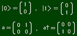
|0> and |1> are the following functions.
φ₀(0) = 1 and φ₀(1) = 0 ・・・ |0>
φ₁(0) = 0 and φ₁(1) = 1 ・・・ |1>

a and a† are the following linear operators.
aφ₀ = 0 and aφ₁ = φ₀,
a†φ₀ = φ₁ and a†φ₁ = 0.

An arbitrary function φ is expressed as
φ = φ(0)φ₀ + φ(1)φ₁
and so
aφ = φ(0)aφ₀ + φ(1)aφ₁ = φ(1)φ₀,
a†φ = φ(0)a†φ₀ + φ(1)a†φ₁ = φ(0)φ₁,
a†aφ = [aφ(0)]φ₁ = φ(1)φ₀(0)φ₁ = φ(1)φ₁
∴ (aφ)(n) = φ(1)φ₀(n) = δ_n0Σ_k=0¹δ_k1φ(k),
　　(a†φ)(n) = φ(0)φ₁(n) = δ_n1Σ_k=0¹δ_k0φ(k),
　　(a†aφ)(n) = φ(1)φ₁(n) = δ_n1φ(1) = δ_n1φ(n).

A quantum history is represented by a functional Φ whose variable is a function n and whose value is a complex number.
Φ[n] ∈ C,
n(t) = 0 or 1,
t ∈ R.

ih lim_ε→+0(1/ε){Φ[n(□ -ε)] - Φ[n]} = cα∫_-∞^∞dt δ_n(t),1Φ[n].

⊿_tΦ[n] ≡ lim_ε→+0(1/ε){Φ[n'] - Φ[n'']},
　t - ε≦ t' ＜ t ⇒ n'(t') = 1 and n''(t') = 0,
　t' ＜ t - ε or t' ≧ t ⇒ n'(t') = n''(t') = n(t').

Φ[n(□ -ε)] - Φ[n] ～ -ε∫_-∞^∞dt [dn(t)/dt]⊿_tΦ[n]
because dn(t)/dt is a sum of delta functions.

-ih∫_-∞^∞dt [dn(t)/dt]⊿_tΦ[n] = cα∫_-∞^∞dt δ_n(t),1Φ[n].
∴∫_-∞^∞dt {ih[dn(t)/dt]⊿_t + cαδ_n(t),1]Φ[n]
　　witten at 2019/04/18/14:57.

On the other hand, the Schrodinger equation of the same system in the old grammar is derived as follows.

ih(∂/∂t)[φ(0, t)|0> + φ(1, t)|1>] = ca†a[φ(0, t)|0> + φ(1, t)|1>]
∴ ih(∂/∂t)φ(0, t)|0> + ih(∂/∂t)φ(1, t)|1> = cφ(1, t)|1>
∴ ih(∂/∂t)φ(0, t) = 0 and ih(∂/∂t)φ(1, t) = cφ(1, t).

A solution of this set of equations must be as follows.
φ(0, t) = c₁, φ(1, t) = c₂ exp[-(i/h)ct].
The normalization condition fort this solution is as follows.
|φ(0, t)|² + |φ(1, t)|² = 1
∴ |c₁|² + |c₂|² = 1.
I am glad of how plausible this solution is.

-ih∫_-∞^∞dt [dn(t)/dt][⊿/⊿n(t)]Φ[n] = cα∫_-∞^∞dt n(t)Φ[n]
where [⊿/⊿n(t)]Φ[n]≡ lim_ε→+0(1/ε){Φ[n'] - Φ[n'']},
　t - ε≦ t' ＜ t ⇒ n'(t') = 1 and n''(t') = 0,
　t' ＜ t - ε or t' ≧ t ⇒ n'(t') = n''(t') = n(t').
This is a good conclusion for the preparation system.
However, another construction may be possible.
It is as follows.
[a(t), a†(t')]₊ = δ(t - t'),
ih lim_ε→+0(1/ε){Φ[ν(□ -ε)] - Φ[ν]} = cα∫_-∞^∞dt a†(t)a(t)Φ[ν].
This method also realize [a†(t)a(t), a†(t')a(t')]_- = 0 if t ≠ t'.
If I use this method, the eigenvalue ν(t) of a†(t)a(t) is not finite but δ(0).
I want to avoid using such ν.
As for the above preparation system, I can adopt the method using n(t) = 0, 1 described above.
However, for the Dirac field as our goal, the eigenvalue of ψ_α†(x)ψ_α(x) is not finite but δ³(0).
So, for the Dirac field, I can not adopt the method using n(t) = 0, 1 described above.
Moreover, [a(t), a†(t')]₊ = δ(t - t') fits [ψ_α(x)ψ_β†(y)]₊ = δ_αβδ³(x - y) very well.
These conditions can be unified to a four-dimensional form:
[ψ_α(x, t)ψ_β†(y, t')]₊ = δ_αβδ³(x - y)δ(t - t')
or [ψ_α(x)ψ_β†(y)]₊ = δ_αβδ⁴(x - y).
This is an additional advantage.
However, the number of fermions is countable at each time.
This does not fit the fact that the graph of n(t) is drawn only by lines.
To make such graph of n(t), we must let a†(t) operate to the vacuum for continuous interval of t.
We do not yet have a way to write it mathematically.2019/05/02/21:10

A good idea has arised.
Let us define |n> by the following condition.
n(t) = 0 ⇒ a(t)|n> = 0,
n(t) = 1 ⇒ a†(t)|n> = 0.
This definition enables n(t) to be 1 for all t in any continuous part of time axis.
However, a†(t)a(t)|n> = δ(0)|n> if n(t) = 1.
I do not want to use the infinite divergent factor δ(0) which is the value of the delta function at the origin.
Though it is one of eigenvalues of ψ_α†(x)ψ_α(x) in QED, perhaps many theorists do not think of such a factor as acceptable.
So, I try replacing a†(t)a(t)|n> with n(t)|n>.
This prescription brings the following treatment to the Dirac field.
[ψ_α(x, t)ψ_β†(y, t')]₊ = δ_αβδ³(x - y)δ(t - t'),
ρ(x, α, t) = 0 ⇒ ψ_α(x, t)|ρ> = 0,
ρ(y, α, t) = δ³(y - x) ⇒ ψ_α†(x, t)|ρ> = 0,
ψ_α†(x, t)ψ_α(x, t)|ρ> is replaced by ρ(x, α, t)|ρ>.
Here ρ should be understood as a three-dimensional number density.2019/05/03/19:14

ρ(x, α, t) = Σ_k δ_{α, g(t, k)}δ(x¹ - f₁(t, k))δ(x² - f₂(t, k))δ(x³ - f₃(t, k)),
g(t, k) = 0 or 1 or 2 or 3 or 4.
δ_{α, g(t, k)} is not zero for some α only when t obeys g(t, k) ≠ 0.
ψ_α†(x, t)ψ_α(x, t)|ρ> = ρ(x, α, t)|ρ>.
ψ_α†(x, t)∂₁ψ_β(x, t)|ρ> = lim_ε→+0(1/ε)(|ρ'> - |ρ''>),
ρ'(x', α', t') = Σ_k δ_{α', g'(t', k)}δ(x'¹ - f'₁(t', k))δ(x'² - f₂(t', k))δ(x'³ - f₃(t', k)),
ρ''(x', α', t') = Σ_k δ_{α', g'(t', k)}δ(x'¹ - f''₁(t', k))δ(x'² - f₂(t', k))δ(x'³ - f₃(t', k)),
g(t, k) ≠ β ⇒ g'(t', k) = g(t', k) and f'₁(t', k) = f₁(t', k).
g(t, k) = β ⇒ [t - ε' ≦ t' ＜ t ⇒ g'(t', k) = α] and [t' ＜ t - ε' or t' ≧ t ⇒ g'(t', k) = g(t', k)].
g(t, k) = β ⇒ [t' ＜ t - ε' or t' ≧ t ⇒ f'₁(t', k) = f₁(t', k)].
g(t, k) = β ⇒ [t' ＜ t - ε' or t' ≧ t ⇒ f''₁(t', k) = f₁(t', k)].
lim_ε→+0ε' → 0.
The area between f'₁(t', k) and f''₁(t', k) is ε in t-f₁ plane.
This idea is difficult to explain linguistically but graphically simple.2019/05/04/21:14

I give graphical representations below.

　

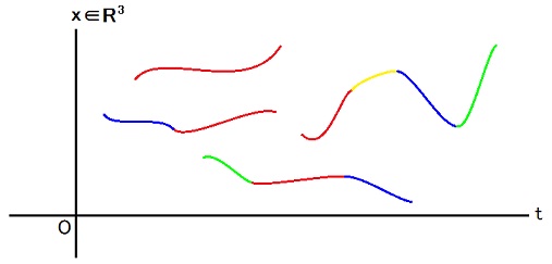
This picture represents the number density function ρ such that
ρ(x, α, t) = Σ_k δ_{α, g(t, k)}δ(x¹ - f₁(t, k))δ(x² - f₂(t, k))δ(x³ - f₃(t, k)),
g(t, k) = 0 or 1 or 2 or 3 or 4.
I want to write f_k¹(t), f_k²(t), f_k³(t), g_k(t) in place of f₁(t, k), f₂(t, k), f₃(t, k), g(t, k).
To avoid halving the size of g_k(t), I have to write g(t, k).
Because I write g(t, k), I should write f₁(t, k), f₂(t, k), f₃(t, k).
k is a name of a curve in the picture.
The k-th curve is expressed by the following set of three equations.
x¹ = f_k¹(t), x² = f_k²(t), x³ = f_k³(t).
g_k(t) corresponds to the color of the point (t, x¹, x², x³) = (t, f_k¹(t), f_k²(t), f_k³(t)) and represents what fermion exists at the point.
If ψ_α†(f_k¹(t), f_k²(t), f_k³(t), t)|ρ> = 0, g_k(t) = α.

α	color in picture
1	red
2	yellow
3	green
4	blue

I have set g_k(t) = 0 for the purpose of terminating the k-th curve.
It works because α≠0.
Please notice that there can be more than one k for a same f because g can differ.
For example,
　

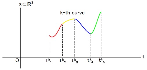
t ＜ t^k₁ ⇒ g_k(t) = 0,
t^k₁ ＜ t ＜ t^k₂ ⇒ g_k(t) = 1,
t^k₂ ＜ t ＜ t^k₃ ⇒ g_k(t) = 2,
t^k₃ ＜ t ＜ t^k₄ ⇒ g_k(t) = 4,
t^k₄ ＜ t ＜ t^k₅ ⇒ g_k(t) = 3,
t ＞ t^k₅ ⇒ g_k(t) = 0.

∫d³x ψ₄†(x, a)∂₂ψ₁(x, a)|ρ> ≡ lim_ε→+0 (1/ε)(|ρ'> - |ρ''>),
　

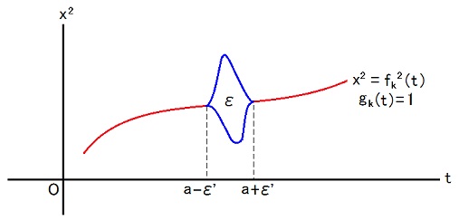
ρ' is made by replacing every a -ε' < t < a +ε' part of each red curve with lower blue curve.
ρ'' is made by replacing every a -ε' < t < a +ε' part of each red curve with upper blue curve.
Only f_k² is deformed and neither f_k³ nor f_k¹ is deformed.
g_k(t) is changed from 1 to 4 only in the part a -ε' < t < a +ε'.
The area between two blue curves has to be ε.
ε' has to be positive and has to tend to zero as ε tends to zero.
As a definition, limit is taken just after replacement for each curve then all results of them are summed.
However, if we replace all necessary parts before subtraction and limitation, the result becomes same because of the character of derivative.2019/05/05/17:55.

f¹(t) is a mapping which maps k on f_k¹(t),
f²(t) is a mapping which maps k on f_k²(t),
f³(t) is a mapping which maps k on f_k³(t),
g(t) is a mapping which maps k on g_k(t),
f(t) is a mapping which maps j on f^j(t),
f is a mapping which maps t on f(t),
g is a mapping which maps t on g(t),
ρ[ f, g ] ∈ R³×{1, 2, 3, 4}×R → R.
{ ρ[ f, g ] }(x, α, t) ≡ Σ_k δ(α, g_k(t))δ(x¹ - f_k¹(t))δ(x² - f_k²(t))δ(x³ - f_k³(t))
　where δ(α, β) ≡ δ_αβ.
{ δ_αβ/[δf^j(t)] } |ρ[ f, g ] > ≡ ∫d³x ψ_α†(x, t)∂_jψ_β(x, t) |ρ[ f, g ] > defined graphically above.

[ { ρ[ f, g ] }(□, □, □ - ε) ] (x, α, t) = { ρ[ f, g ] } (x, α, t - ε)
= Σ_k δ(α, g_k(t - ε))δ(x¹ - f_k¹(t - ε))δ(x² - f_k²(t - ε))δ(x³ - f_k³(t - ε))
= { ρ[ f(□ - ε), g(□ - ε) ] } (x, α, t)
∴ { ρ[ f, g ] }(□, □, □ - ε) = ρ[ f(□ - ε), g(□ - ε) ].

lim_ε→+0 (1/ε) [ | {ρ[ f, g ] } (□, □, □ - ε) > - |ρ[ f, g ] > ].
= -∫_-∞^∞dt Σ_k{Σ_j=1³[df_k^j(t)/dt][δ/δf_k^j(t)] + [dg_k(t)/dt][⊿/⊿g_k(t)] }|ρ[ f, g ] >.

Uda Equation:
-ih∫_-∞^∞dt Σ_k{Σ_j=1³[df_k^j(t)/dt][δ/δf_k^j(t)] + [dg_k(t)/dt][⊿/⊿g_k(t)] } Φ[ f, g ]
　= α∫_-∞^∞dt { iΣ_α=1⁴Σ_β=1⁴ (γ⁰γ^j)_αβ { δ_αβ/[δf^j(t)] }
　　　　+ m∫d³x [ {ρ[ f, g ] }(x, 1, t) + {ρ[ f, g ] }(x, 2, t) - {ρ[ f, g ] }(x, 3, t) - {ρ[ f, g ] }(x, 4, t) ] }.2019/05/06/17:40

In the above expression, I missed the last factor.
The first term of the integrand in the right hand side of the above equation has the opposite sign to the sign of the corresponding term in the original Hamiltonian.
This is not a mistake because partial integration was done.
The corrected expression of Uda equation of the free Dirac field is as follows.

-ih∫_-∞^∞dt Σ_k{Σ_j=1³[df_k^j(t)/dt][δ/δf_k^j(t)] + [dg_k(t)/dt][⊿/⊿g_k(t)] } Φ[ f, g ]
　= α∫_-∞^∞dt { iΣ_j=1³Σ_α=1⁴Σ_β=1⁴ (γ⁰γ^j)_αβ { δ_αβ/[δf^j(t)] }
　　　　　　　　　　　+ m∫d³x [ {ρ[ f, g ] }(x, 1, t) + {ρ[ f, g ] }(x, 2, t)
　　　　　　　　　　　　　　　　　　　- {ρ[ f, g ] }(x, 3, t) - {ρ[ f, g ] }(x, 4, t) ] }Φ[ f, g ].

　

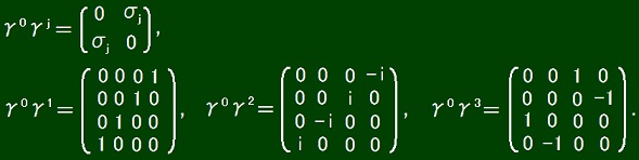
By using these components of the matrices, Uda equation of the free Dirac field is written as follows.

-ih∫_-∞^∞dt Σ_k{Σ_j=1³[df_k^j(t)/dt][δ/δf_k^j(t)] + [dg_k(t)/dt][⊿/⊿g_k(t)] } Φ[ f, g ]
　= α∫_-∞^∞dt { iδ₁₄/[δf¹(t)] + iδ₂₃/[δf¹(t)] + iδ₃₂/[δf¹(t)] + iδ₄₁/[δf¹(t)]
　　　　　　　　　　　+ δ₁₄/[δf²(t)] - δ₂₃/[δf²(t)] + δ₃₂/[δf²(t)] - δ₄₁/[δf²(t)]
　　　　　　　　　　　+ iδ₁₃/[δf³(t)] - iδ₂₄/[δf³(t)] + iδ₃₁/[δf³(t)] - iδ₄₂/[δf³(t)]
　　　　　　　　　　　+ m∫d³x [ {ρ[ f, g ] }(x, 1, t) + {ρ[ f, g ] }(x, 2, t)
　　　　　　　　　　　　　　　　　　　- {ρ[ f, g ] }(x, 3, t) - {ρ[ f, g ] }(x, 4, t) ] }Φ[ f, g ].
2019/05/07/15:20.

The above expression still includes mistakes.
Σ_ρΦ[ρ] ( |ρ'> - |ρ''> ) = Σ_ρ{ Φ[ 'ρ] - Φ[ ''ρ] } |ρ>.
'ρ is made by letting the inverse operator operate to ρ compared to the operator used to make ρ' from ρ.
''ρ is made by letting the inverse operator operate to ρ compared to the operator used to make ρ'' from ρ.
2019/05/09/17:47.

For two days, I have tried to think out the way how to make 'ρ and ''ρ from ρ.
The crime for example letting me hear various noises to prevent me from thinking is being done by humble people operated by my inferior rivals.
So, I meditated in a lying pose on my bed.
Today(2019/05/11), I noticed that I may go further when I use Fock representation.

One of basis of Fock representation u is a function such that:
u(x₁, α₁; ・・・; x_n, α_n)
　= Σ_πsgn(π)δ³(x_π(1) - a₁)δ(α_π(1), A₁) ・・・ δ³(x_π(n) - a_n)δ(α_π(n), A_n)

[∫d³x ψ_α†(x)∂_jψ_β(x)] u(x₁, α₁; ・・・; x_n, α_n)
　= - (∂/∂x^j)Σ_k=1ⁿΣ_πsgn(π)δ³(x_π(1) - a₁)δ(α_π(1), A₁) ・・・ δ³(x_π(k) - x)δ(α_π(k), α) ・・・ δ³(x_π(n) - a_n)δ(α_π(n), A_n)
　= Σ_k=1ⁿΣ_πsgn(π)(∂/∂x_π(k)^j)δ³(x_π(1) - a₁)δ(α_π(1), A₁) ・・・ δ³(x_π(k) - x)δ(α_π(k), α) ・・・ δ³(x_π(n) - a_n)δ(α_π(n), A_n).
2019/05/11/19:35

I noticed that the above expression is wrong.
[Σ_β=1⁴Σ_β'=1⁴∫d³x ψ_β†(x)(γ⁰γ^j)_ββ'∂_jψ_β'(x)] u(x₁, α₁; ・・・; x_n, α_n)
　= - Σ_k=1ⁿΣ_β=1⁴(γ⁰γ^j)_βA(k)(∂/∂a_k^j)Σ_πsgn(π)δ³(x_π(1) - a₁)δ(α_π(1), A₁) ・・・ δ³(x_π(k) - a_k)δ(α_π(k), β) ・・・ δ³(x_π(n) - a_n)δ(α_π(n), A_n)
　= Σ_k=1ⁿΣ_πsgn(π)(∂/∂x_π(k)^j)δ³(x_π(1) - a₁)δ(α_π(1), A₁) ・・・ (γ⁰γ^j)_{α(π(k)),A(k)}δ³(x_π(k) - a_k) ・・・ δ³(x_π(n) - a_n)δ(α_π(n), A_n)
　= Σ_k=1ⁿ(∂/∂x_k^j)Σ_β=1⁴(γ⁰γ^j)_α(k),βu(x₁, α₁; ・・・; x_k, β; x_n, α_n).
How is this which gives us a great hint?
2019/05/12/14:18

Below I verify and explain the above expression.

[ψ_α†(x)ψ_β(y)]ψ_A†(a) = ψ_α†(x)[δ_βAδ³(y - a) - ψ_A†(a)ψ_β(y)]
　= δ_βAδ³(y - a)ψ_α†(x) + ψ_A†(a)ψ_α†(x)ψ_β(y)
∴ [ψ_α†(x)ψ_β(y), ψ_A†(a)]_- = δ_βAδ³(y - a)ψ_α†(x).

[ψ_α†(x)ψ_β(y)]ψ_A(1)†(a₁)ψ_A(2)†(a₂)ψ_A(3)†(a₃)|0>
= [ψ_α†(x)ψ_β(y), ψ_A(1)†(a₁)]_-ψ_A(2)†(a₂)ψ_A(3)†(a₃)|0>
　　+ ψ_A(1)†(a₁)[ψ_α†(x)ψ_β(y)]ψ_A(2)†(a₂)ψ_A(3)†(a₃)|0>
= [ψ_α†(x)ψ_β(y), ψ_A(1)†(a₁)]_-ψ_A(2)†(a₂)ψ_A(3)†(a₃)|0>
　　+ ψ_A(1)†(a₁)[ψ_α†(x)ψ_β(y), ψ_A(2)†(a₂)]_-ψ_A(3)†(a₃)|0>
　　+ ψ_A(1)†(a₁)ψ_A(2)†(a₂)[ψ_α†(x)ψ_β(y)]ψ_A(3)†(a₃)|0>
= [ψ_α†(x)ψ_β(y), ψ_A(1)†(a₁)]_-ψ_A(2)†(a₂)ψ_A(3)†(a₃)|0>
　　+ ψ_A(1)†(a₁)[ψ_α†(x)ψ_β(y), ψ_A(2)†(a₂)]_-ψ_A(3)†(a₃)|0>
　　+ ψ_A(1)†(a₁)ψ_A(2)†(a₂)[ψ_α†(x)ψ_β(y), ψ_A(3)†(a₃)]_-|0>
　　+ ψ_A(1)†(a₁)ψ_A(2)†(a₂)ψ_A(3)†(a₃)[ψ_α†(x)ψ_β(y)]|0>
= δ_βA(1)δ³(y - a₁)ψ_α†(x)ψ_A(2)†(a₂)ψ_A(3)†(a₃)|0>
　　+ ψ_A(1)†(a₁)δ_βA(2)δ³(y - a₂)ψ_α†(x)ψ_A(3)†(a₃)|0>
　　+ ψ_A(1)†(a₁)ψ_A(2)†(a₂)δ_βA(3)δ³(y - a₃)ψ_α†(x)|0>.

[ψ_α†(x)ψ_β(y)]ψ_A(1)†(a₁) ・・・ ψ_A(n)†(a_n)|0>
= Σ_k=1ⁿδ_βA(k)δ³(y - a_k)ψ_A(1)†(a₁) ・・・ ψ_A(k-1)†(a_k-1)ψ_α†(x)ψ_A(k+1)†(a_k+1) ・・・ ψ_A(n)†(a_n)|0>.

[ψ_α†(x)ψ_β(x + εδ_□j)]ψ_A(1)†(a₁) ・・・ ψ_A(n)†(a_n)|0>
= Σ_k=1ⁿδ_βA(k)δ³(x + εδ_□j - a_k)ψ_A(1)†(a₁) ・・・ ψ_A(k-1)†(a_k-1)ψ_α†(x)ψ_A(k+1)†(a_k+1) ・・・ ψ_A(n)†(a_n)|0>.

∫d³x [ψ_α†(x)ψ_β(x + εδ_□j)]ψ_A(1)†(a₁) ・・・ ψ_A(n)†(a_n)|0>
= Σ_k=1ⁿδ_βA(k)ψ_A(1)†(a₁) ・・・ ψ_A(k-1)†(a_k-1)ψ_α†(a_k - εδ_□j)ψ_A(k+1)†(a_k+1) ・・・ ψ_A(n)†(a_n)|0>.

∫d³x [ψ_α†(x)∂_jψ_β(x)]ψ_A(1)†(a₁) ・・・ ψ_A(n)†(a_n)|0>
= lim_ε→0(1/ε)∫d³x [ψ_α†(x)ψ_β(x + εδ_□j)]ψ_A(1)†(a₁) ・・・ ψ_A(n)†(a_n)|0>
= -Σ_k=1ⁿ(∂/∂a_k^j)δ_βA(k)ψ_A(1)†(a₁) ・・・ ψ_A(k-1)†(a_k-1)ψ_α†(a_k)ψ_A(k+1)†(a_k+1) ・・・ ψ_A(n)†(a_n)|0>.

Σ_α=1⁴Σ_β=1⁴(γ⁰γ^j)_αβ∫d³x [ψ_α†(x)∂_jψ_β(x)]ψ_A(1)†(a₁) ・・・ ψ_A(n)†(a_n)|0>
= -Σ_k=1ⁿ(∂/∂a_k^j)Σ_α=1⁴(γ⁰γ^j)_αA(k)ψ_A(1)†(a₁) ・・・ ψ_A(k-1)†(a_k-1)ψ_α†(a_k)ψ_A(k+1)†(a_k+1) ・・・ ψ_A(n)†(a_n)|0>.

In the Fock representation, state ψ_A(1)†(a₁) ・・・ ψ_A(n)†(a_n)|0> is represented by a wave function such that
u(x₁, α₁; ・・・; x_n, α_n) = Σ_πsgn(π)δ(α_π(1), A₁)δ³(x_π(1) - a₁) ・・・ δ(α_π(n), A_n)δ³(x_π(n) - a_n).

So, Fock representation of operator Σ_β=1⁴Σ_β'=1⁴(γ⁰γ^j)_ββ'∫d³y [ψ_β†(y)∂_jψ_β'(y)] is as
Σ_β=1⁴Σ_β'=1⁴(γ⁰γ^j)_ββ'∫d³y [ψ_β†(y)∂_jψ_β'(y)]u(x₁, α₁; ・・・; x_n, α_n)
= -Σ_k=1ⁿ(∂/∂a_k^j)Σ_β=1⁴(γ⁰γ^j)_βA(k)Σ_πsgn(π)δ(α_π(1), A₁)δ³(x_π(1) - a₁) ・・・ δ(α_π(k), β)δ³(x_π(k) - a_k) ・・・ δ(α_π(n), A_n)δ³(x_π(n) - a_n)
= -Σ_k=1ⁿ(∂/∂a_k^j)Σ_πsgn(π)δ(α_π(1), A₁)δ³(x_π(1) - a₁) ・・・ (γ⁰γ^j)_{α(π(k))A(k)}δ³(x_π(k) - a_k) ・・・ δ(α_π(n), A_n)δ³(x_π(n) - a_n)
= Σ_πsgn(π)Σ_k=1ⁿ(∂/∂x_π(k)^j)Σ_α'=1⁴(γ⁰γ^j)_α(π(k))α'δ(α_π(1), A₁)δ³(x_π(1) - a₁) ・・・ δ(α', A_k)δ³(x_π(k) - a_k) ・・・ δ(α_π(n), A_n)δ³(x_π(n) - a_n)
= Σ_k=1ⁿ(∂/∂x_k^j)Σ_α'=1⁴(γ⁰γ^j)_α(k)α'u(x₁, α₁; ・・・; x_k-1, α_k-1; x_k, α'; x_k+1, α_k+1; ・・・; x_n, α_n).

For a general n-particles wave-function F, I assume that
Σ_β=1⁴Σ_β'=1⁴(γ⁰γ^j)_ββ'∫d³y [ψ_β†(y)∂_jψ_β'(y)]F(x₁, α₁; ・・・; x_n, α_n)
= Σ_k=1ⁿ(∂/∂x_k^j)Σ_β=1⁴(γ⁰γ^j)_α(k)βF(x₁, α₁; ・・・; x_k-1, α_k-1; x_k, β; x_k+1, α_k+1; ・・・; x_n, α_n).
2019/05/14/18:05

By depending on this result for quantum state, I may be able to assume how Hamiltonian operates to a quantum history.
However, I wonder how to realize antisymmetricity of a functional representing a quantum history though I know how to realize antisymmetricity of a function representing a quantum state.

For an unentangled quantum history in time-like direction, quantum state at time t is replaced by a quantum state at time t + ε for all t if α∫dt∫d³xψ†(x, t)ψ(x, t + ε) operates to the quantum history.
So, the difference between such a quantum history and a quantum history before replacement is
α[∫dt∫d³xψ†(x, t)ψ(x, t + ε) - ∫dt∫d³xψ†(x, t)ψ(x, t)] |quantum history vector>.

ih lim_ε→0(1/ε)α[∫dt∫d³xψ†(x, t)ψ(x, t + ε) - ∫dt∫d³xψ†(x, t)ψ(x, t)]
= ihα∫dt∫d³xψ†(x, t)(∂/∂t)ψ(x, t)
= ihα∫d(ct)∫d³xψ†(x, t)[∂/∂(ct)]ψ(x, t)
= ihα∫d⁴xψ†(x)(∂/∂x⁰)ψ(x)
= ihα∫d⁴xψ†(x)∂₀ψ(x)
= ∫d⁴xψ†(x)γ⁰[ ihαγ⁰∂₀]ψ(x) ∵ γ⁰γ⁰ = 1.

H(t) = ∫d³x ψ†(x, t)γ⁰(-ihcγ^k∂_k + mc²)ψ(x, t).
α∫dt H(t) = α∫dt∫d³x ψ†(x, t)γ⁰(-ihcγ^k∂_k + mc²)ψ(x, t)
= ∫d(ct)∫d³x ψ†(x, t)γ⁰(-ihαγ^k∂_k + mcα)ψ(x, t)
= ∫d⁴x ψ†(x)γ⁰(-ihαγ^k∂_k + mcα)ψ(x)

Uda Equation:
∫d⁴xψ†(x)γ⁰[ ihαγ⁰∂₀]ψ(x) |quantum history vector>
= ∫d⁴x ψ†(x)γ⁰(-ihαγ^k∂_k + mcα)ψ(x) |quantum history vector>
∴ ∫d⁴x ψ†(x)γ⁰(-ihαγ^μ∂_μ + mcα)ψ(x) |quantum history vector> = 0.
∴ ∫d⁴x ψ†(x)γ⁰(-ihγ^μ∂_μ + mc)ψ(x) |quantum history vector> = 0.

More explicitly
∫d⁴xΣ_α=1⁴Σ_β=1⁴ψ_α†(x)[-ihΣ_μ=0³(γ⁰γ^μ)_αβ∂_μ + mc(γ⁰)_αβ]ψ_β(x) |quantum history vector> = 0.
[ψ_α(x), ψ_β†(y)]₊ = δ_αβδ⁴(x - y), [ψ_α(x), ψ_β(y)]₊ = 0.
This is the operator form of Uda equation of free Dirac field.
I wrote a memo of this in 15th @ May 2019 @ News.
I am surprised at how plausible this expression is and glad of it while I wonder what the maze before it was.
I worry that this equation might contradict to existing quantum theory of Dirac field.
I also worry about disappearing of factor α.
Without this factor, my theory can not be a correction to the existing theory but only be a direct denial of the existing theory.
It worries me because the existing theory is strongly supported by experimental evidences.

Author Yuichi Uda, Write start at 2019/04/15/19:09JST, Last edit at 2019/05/15/17:47JST